Functions
Operators
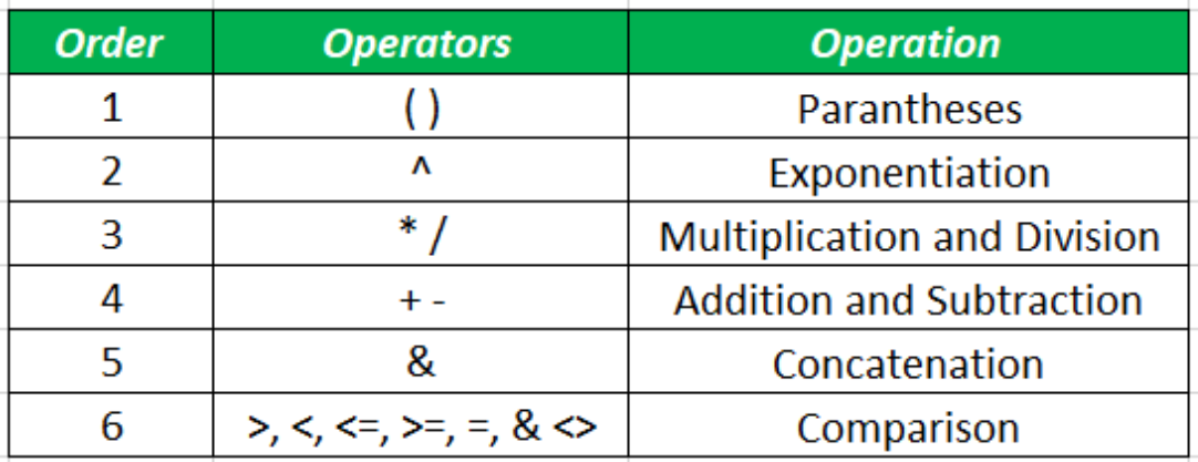
Arithmetic Operators
Performed in the BODMAS arithmetic operator precedence.
Examples:
- Addition:
=A2+A3 - Subtraction:
=A2-A3 - Multiplication:
=A2*A3 - Division:
=A2/A3 - Indices:
=A2^A3
Logical Operators
Can be found under the Conditionals section
SUM
Learn more:
SUM
Syntax: =SUM(cell1:cell2)
Summary: Sum/total of everything in range from cell1 to cell2.
Paramaters:
cell1:cell2- is called a cell reference.
SUMIF
Syntax: =SUMIF(range, criteria, [sum_range])
Summary: Sum if the given one criteria is met.
Paramaters:
range- where your criteria sits
criteria- what to search for
- eg:
32,"32",">32","Sales"
[sum_range]- optional
- not used if we are going to sum the criteria range
- eg: when comparing numbers.
- numbers to sum if condition met, from same table.
- optional
Examples:
=SUMIF(c1:c9, ">1500")
- sum salaries
- if salary is more than
1500
=SUMIF(c1:c9, "<1500")
- sum salaries
- if salary is less than
1500
=SUMIF(a1:a9, "Sales", c1:c9)
- explanation 1
a1:a9is job descriptions- if job description is
"Sales" - then, sum
c1:c9
- explanation 2
a1:a9is job descriptionsc1:c9is their salaries- sum the salaries of people in Sales
SUMIFS
Syntax: =SUMIF(sum_range, criteria_range1, criteria1, [criteria_range2, criteria2], ...)
Summary: Sum if multiple conditions are met
Paramaters:
sum_range- range of cells to sum from
- if conditions are met
criteria_range1- where to look for the first condition
criteria1- first condition
criteria_range2- where to look for the second condition
criteria2- second condition
- can have 127
criteria_rangeXandcriteriaX
Examples:
a1:a9is job descriptionsb1:b9is genderc1:c9is salary
=SUMIFS(c1:c9, a1:a9, "Sales", b1:b9, "Female")
- sum salaries in
c1:c9 - if person in Sales (if "
Sales" ina1:a9) and - if person is Female (if "
Female" inb1:b9) - (sum of salaries of every female working in Sales)
=SUMIFS(c1:c9, a1:a9, "Sales", b1:b9, "Female", c1:c9, ">1500")
- sum salaries in
c1:c9 - if person in Sales (if "
Sales" ina1:a9) and - if person is Female (if "
Female" inb1:b9) and - if person's salary is greater than 1500 (if
c1:c9is>1500) - (sum of salaries of every female working in Sales who earns more than 1500)
COUNT
Learn more:
COUNT
Syntax: =COUNT(range, [range2], ...)
Summary: Count the number of cells with numbers only
Parameters:
range- a cell range reference
- eg:
c1:c9
[range2]- other ranges to count from
Examples:
=COUNT(c1:c9)
- the number of cells with numbers in range
c1:c9 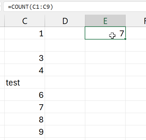
- not 9, its 7
- two cells are not counted
- 2nd cell: empty
- 5th cell: has text (not a number)
COUNTA
Syntax: =COUNTA(range, [range2], ...)
Summary: Count the number of cells with both numbers and letters (alpha characters) only. Bascially alpha-numeric.
Parameters:
range- a cell range reference
- eg:
c1:c9
[range2]- other ranges to count from
Examples:
=COUNTA(c1:c9)
- the number of cells with both numbers and letters
- in range
c1:c9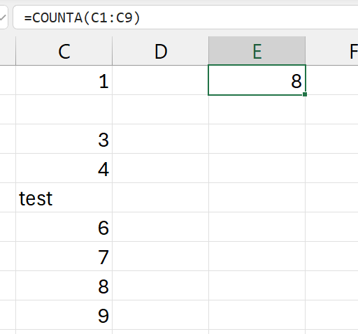
- in range
- only one cell is not counted
- 2nd cell: empty
- the 5th cell is counter, because its alpha-numeric (has letters).
=COUNTA(c1:c9, b1:b9)
- the number of cells with both numbers and letters
- in ranges
c1:c9 - and range
b1:b9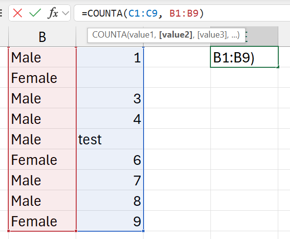
- in ranges
- answer is
179(fromb1:b9)- everything is counted
- +
8(fromc1:c9)- only the empty cell is not counted
- everything else is counted
9 + 8 = 17
COUNTBLANK
Syntax: =COUNTBLANK(range)
Summary: Count the number of empty/blank cells.
Parameters:
range- a cell range reference
- eg:
c1:c9
Examples:
=COUNTBLANK(c1:c9)
- the number of blank cells
- in range:
c1:c9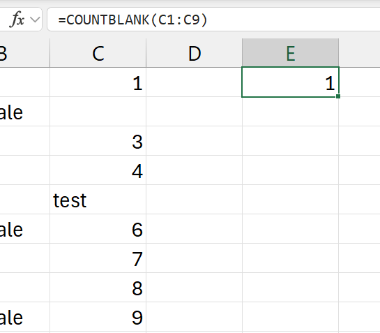
- in range:
- only the cell is 2nd row is empty
COUNTIF
Syntax: =COUNTIF(range, criteria)
Summary: Count the number of cells that meets the given condition from the given range
Parameters:
range- a cell range reference
- eg:
c1:c9
criteria- the condition to meet to count
Examples:
a1:a9is job descriptionsb1:b9is genderc1:c9is salary
=COUNTIF(c1:c9, ">1500")
- count number of cells (people)
- that earns more than "
>1500"
=COUNTIF(b1:b9, "Female")
- count the number of cells (people)
- if gender is "Female"
- basically, the number of female employees
COUNTIFS
Syntax: =COUNTIFS(range, criteria, [range2, criteria2], ...)
Summary: Count the number of cells that meets the given condition from the given range
Parameters:
range- a cell range reference
- eg:
c1:c9
criteria- the condition to meet for
range
- the condition to meet for
range2- a cell range reference
- eg:
b1:b9
criteria2- the condition to meet for
range2
- the condition to meet for
- can have as many
rangeXandcriteriaXas possible
Examples:
a1:a9is job descriptionsb1:b9is genderc1:c9is salary
=COUNTIFS(b1:b9, "Female", c1:c9, ">1500")
- count of cells (people)
- where gender is Female
- where salary is greater than 1500
- basically, females who earn more than 1500
=COUNTIFS(a1:a9, "Sales", b1:b9, "Female", c1:c9, ">1500")
- count of cells (people)
- where job description is Sales
- where gender is Female
- where salary is greater than 1500
- basically, females working in Sales who earn more than 1500
AVERAGE
Learn more:
AVERAGE
Syntax: =AVERAGE(range, [range2], ...)
Summary: Average of everything in the selected range(s).
Paramaters:
range- range to calculate average of.
- eg:
c1:c9
[range2]- other ranges to calculate average of
Examples:
a1:a9is job descriptionsb1:b9is genderc1:c9is salaryd1:d9is bonus
=AVERAGE(c1:c9)
- average of all numerical values in range
c1:c9
=AVERAGE(c1:c9, d1:d9)
- average of all numerical values
- in range
c1:c9 - and range
d1:d9
- in range
AVERAGEIF
Syntax: =AVERAGEIF(range, criteria, [average_range])
Summary: Average of everything in the selected range(s).
Paramaters:
range- is called a cell reference.
- eg:
c1:c9
criteria- condition to check in
range
- condition to check in
[average_range]- optional
- not used if we are going to sum the criteria range
- when comparing numbers
- numbers to average if condition is met, from same table.
- optional
Examples:
a1:a9is job descriptionsb1:b9is genderc1:c9is salaryd1:d9is bonus
=AVERAGEIF(c1:c9, ">1500")
- calculate average of salaries
- if salary is greater than 1500
=AVERAGEIF(c1:c9, ">1500", d1:d9)
- calculate average of bonuses
- if person's salary is greater than 1500
=AVERAGEIF(a1:a9, "Sales", c1:c9)
- calculate average of salaries
- if person works in Sales
AVERAGEIFS
Syntax: =AVERAGEIFS(average_range, criteria_range1, criteria1, [criteria_range2, criteria2], ...)
Summary: Average if multiple conditions are met
Paramaters:
average_range- range of cells to average from
- if conditions are met
criteria_range1- where to look for the first condition
criteria1- first condition
criteria_range2- where to look for the second condition
criteria2- second condition
- can have 127
criteria_rangeXandcriteriaX
Examples:
a1:a9is job descriptionsb1:b9is genderc1:c9is salaryd1:d9is bonus
=AVERAGEIFS(c1:c9, a1:a9, "Sales", b1:b9, "Female")
- average salaries in
c1:c9 - if person in Sales (if "
Sales" ina1:a9) and - if person is Female (if "
Female" inb1:b9) - (average of salaries of every female working in Sales)
=AVERAGEIFS(c1:c9, a1:a9, "Sales", b1:b9, "Female", c1:c9, ">1500")
- average salaries in
c1:c9 - if person in Sales (if "
Sales" ina1:a9) and - if person is Female (if "
Female" inb1:b9) and - if person's salary is greater than 1500 (if
c1:c9is>1500) - (average of salaries of every female working in Sales who earns more than 1500)
MIN
MIN
Syntax: =MIN(range, [range2], ...)
Summary: Get the minimum value of everything in the selected range(s) with numerical values.
Paramaters:
range- range to find minimum value of.
- should only have numerican data values
- eg:
c1:c9
[range2]- other ranges with numerical vata to find minimum value of
Examples:
=MIN(c1:c9)
- minimum numerical value in cell range
c1:c9
=MIN(c1:c9, d1:d9)
- minimum numerical value
- in cell range
c1:c9 - and
d1:d9
- in cell range
MINA
No idea about this.
MINIFS
Syntax: =MINIFS(min_range, criteria_range1, crtieria1, [criteria_range2, crtieria2], ...)
Summary: Get the minimum value of everything in the selected range(s) with numerical values if given conditions are met.
Paramaters:
min_range- cell range to select minimum value from
criteria_range1- where to look for first condition
criteria1- first condition
criteria_range2- where to look for the second condition
criteria2- second condition
- can have 127
criteria_rangeXandcriteriaX
Examples:
a1:a9is job descriptionsb1:b9is genderc1:c9is salaryd1:d9is bonus
=MINIFS(C1:C9, A1:A9, "Tech")
- minimum value in range
C1:C9 - if department is Tech (
A1:A9vale in Tech) - (minimum salary of a Tech employee)
=MINIFS(C1:C9, A1:A9, "Tech", D1:D9, ">1500")
- minimum value in range
C1:C9 - if department is Tech (
A1:A9value in Tech) - if bonus is greater than 1500 (in range
D1:D9) - (minimum salary of a Tech employee if bonus is greater than 1500)
MAX
MAX
Syntax: =MAX(range, [range2], ...)
Summary: Get the maximum value of everything in the selected range(s) with numerical values.
Paramaters:
range- range to find maximum value of.
- should only have numerican data values
- eg:
c1:c9
[range2]- other ranges with numerical vata to find maximum value of
Examples:
=MAX(c1:c9)
- maximum numerical value in cell range
c1:c9
=MAX(c1:c9, d1:d9)
- maximum numerical value
- in cell range
c1:c9 - and
d1:d9
- in cell range
MAXA
No idea about this.
MAXIFS
Syntax: =MAXIFS(min_range, criteria_range1, crtieria1, [criteria_range2, crtieria2], ...)
Summary: Get the maximum value of everything in the selected range(s) with numerical values if given conditions are met.
Paramaters:
min_range- cell range to select maximum value from
criteria_range1- where to look for first condition
criteria1- first condition
criteria_range2- where to look for the second condition
criteria2- second condition
- can have 127
criteria_rangeXandcriteriaX
Examples:
a1:a9is job descriptionsb1:b9is genderc1:c9is salaryd1:d9is bonus
=MAXIFS(C1:C9, A1:A9, "Tech")
- maximum value in range
C1:C9 - if department is Tech (
A1:A9vale in Tech) - (maximum salary of a Tech employee)
=MAXIFS(C1:C9, A1:A9, "Tech", D1:D9, ">1500")
- maximum value in range
C1:C9 - if department is Tech (
A1:A9value in Tech) - if bonus is greater than 1500 (in range
D1:D9) - (maximum salary of a Tech employee if bonus is greater than 1500)
MAX
ROUND
ROUND
Syntax: =ROUND(number, num_digits)
Summary: Rounds the decimal places of a number by the specified number
Paramaters:
number- a number
- a cell reference containing a number
num_digits- number of decimal places
- to round off to
Examples:
c1has 14.7261
=ROUND(c1, 2) or =ROUND(14.7261, 2)
- result:
14.73 num_digitsis 2, so, rounds off to 2 decimal places
ROUNDUP
Syntax: =ROUNDUP(number, num_digits)
Summary: Rounds a number up.
number- a number
- a cell reference containing a number
num_digits- number of decimal places
- to round up to
Examples:
c1has 14.7261
=ROUNDUP(c1, 1) or =ROUNDUP(14.7261, 1)
- result:
14.8 num_digitsis 1, so, rounds up to 1 decimal places
For easy understanding, consider the set of examples below:
=ROUNDUP(13.9, 0)--->14=ROUNDUP(14.0, 0)--->14=ROUNDUP(14.1, 0)--->15- and
=ROUNDUP(14.1, 1)--->14.1=ROUNDUP(14.11, 1)--->14.2=ROUNDUP(14.12, 1)--->14.2- ...
=ROUNDUP(14.19, 1)--->14.2=ROUNDUP(14.2, 1)--->14.2=ROUNDUP(14.21, 1)--->14.3- ...
=ROUNDUP(14.13, 2)--->14.13=ROUNDUP(14.131, 2)--->14.14
ROUNDDOWN
Syntax: =ROUNDDOWN(number, num_digits)
Summary: Rounds a number down
number- a number
- a cell reference containing a number
num_digits- number of decimal places
- to round down to
Examples:
c1has 14.7261
=ROUNDDOWN(c1, 1) or =ROUNDDOWN(14.7261, 1)
- result:
14.7 num_digitsis 1, so, rounds down to 1 decimal places
For easy understanding, consider the set of examples below:
=ROUNDDOWN(13.9, 0)--->13=ROUNDDOWN(14.0, 0)--->14=ROUNDDOWN(14.1, 0)--->14- and
=ROUNDDOWN(14.1, 1)--->14.1=ROUNDDOWN(14.11, 1)--->14.1=ROUNDDOWN(14.12, 1)--->14.1- ...
=ROUNDDOWN(14.19, 1)--->14.1=ROUNDDOWN(14.2, 1)--->14.2=ROUNDDOWN(14.21, 1)--->14.2- ...
=ROUNDDOWN(14.13, 2)--->14.13=ROUNDDOWN(14.131, 2)--->14.13
Conditionals
Of course! these can be nested in whatever the way you want.
OR
Syntax: =OR(condition1, condition3, [condition3], ...)
Summary: Returns TRUE if atleast one condition is TRUE (even if all others are FALSE - except one). If all conditions are FALSE, return FALSE. Basically the OR operator.
Parameters:
conditionX- conditions
AND
Syntax: =AND(condition1, condition3, [condition3], ...)
Summary: Returns TRUE only if all conditions are TRUE. Otherwise, returns False. Basically the AND operator.
Parameters:
conditionX- conditions
NOT
Syntax: =NOT(condition)
Summary: Evaluvate the condition and return the oppsite of the result. If the result is TRUE, this will return FALSE and vice versa. Basically the NOT operator.
Parameters:
condition- a condition
- to be evaluvated
IF (Basic)
Syntax: =IF(logical_test, value_if_true, value_if_false)
Summary: A conditional. Evaluvate logical_test, if its TRUE: return value_if_true and if its FALSE: return: value_if_false
Parameters:
logical_test- condition(al) to be evaluvates
value_if_true- this will be returned
- if the condition is TRUE
value_if_false- this will be returned
- if the condition is FALSE
Example:
=IF(B2=C2, "Yes. Correct!", "No! Wrong")
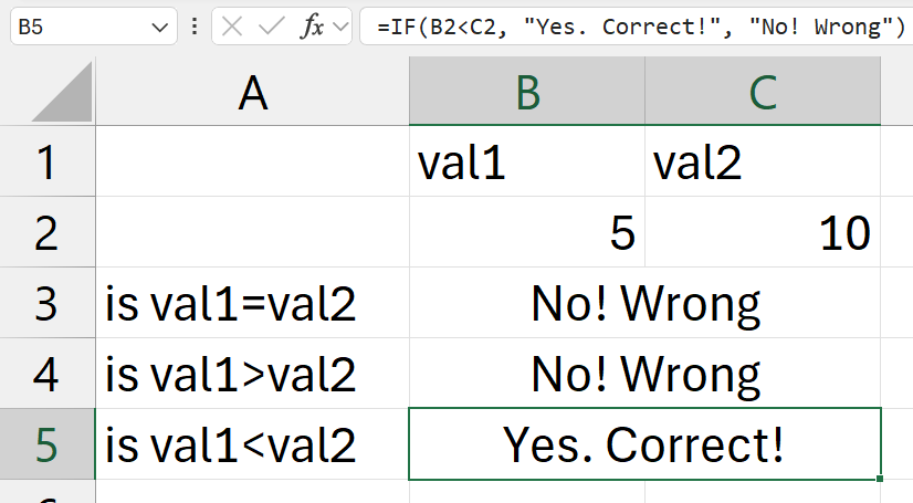
- check if
B2=C2is true?- (is contents of
B2cell equal to contents ofC2cell) - it its correct
- return "
Yes. Correct!"
- return "
- if its wrong
- return "
No! Wrong"
- return "
- (is contents of
IFS
Learn more:
Syntax: =IFS(condition1, result1, [condition2, result2], ...)
Summary: Basically a if-elif-else scenario.
Parameters:
condition1- The condition you want to test
result1- The value that is returned
- if corresponding condition is TRUE
- can have 127
conditionXandresultX
Examples:
=IFS(A4="Apple", "Fruit", A4="Potato", "Vegetable")
- if cell contents equal to "Apple"
- return "Fruit"
- if cell contents equal to "Potato"
- return "Vegetable"
- no ELSE condition
#N/Awill be returned
=IFS(A4="Apple", "Fruit", A4="Potato", "Vegetable", TRUE, "Other")
- if cell contents equal to "Apple"
- return "Fruit"
- if cell contents equal to "Potato"
- return "Vegetable"
- else
- (from the
TRUE, "Other"part) - if no condition is met
- return "Other"
- (from the
IF (Nested)
=IF(condition1, true_result1, IF(condition2, true_result2, false_else_final))
OR
=IF(condition1, true_result1,
    IF(condition2, true_result2,
        IF(condition3, true_result3, false_else_final)
    )
)
is similiar to
=IFS(condition1, true_result1, condition2, true_result2, TRUE, false_else_final)
Errors
IFNA
Syntax: =IFNA(value, value_if_na)
Summary: Returns the value you specify if expression resolves to #N/A, otherwise, return the result of the expression.
Parameters:
value- value (mostly from a function)
- which might return
#N/A- eg:
IFSwithout an else part
- eg:
- if its
#N/A- show
value_if_na
- show
- else
- show the
value
- show the
value_if_na- returned if
valuereturns#N/A
- returned if
Example:
=IFS(condition1, true_result1, condition2, true_result2, TRUE, false_else_final)
is equal to
=IFNA(IFS(condition1, true_result1, condition2, true_result2), false_else_final)
IFERROR
Syntax: =IFERROR(value, value_if_error)
Summary: Returns the value you specify if expression is an error and the value of the expression itself otherwise
value- value (mostly from a function)
- which might raise an error
- eg: mistyped function names
- if it raises an error
- show
value_if_error
- show
- else
- show the
value
- show the
value_if_error- returned if
valueraises an error
- returned if
Example:
=IFERROR(A1, "oops")
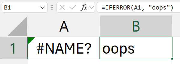
- (where
A1has an error (mistyped function name - no such function exists)) - since A1 has
A1has an error:#NAME? - the text:
oopswill be displayed
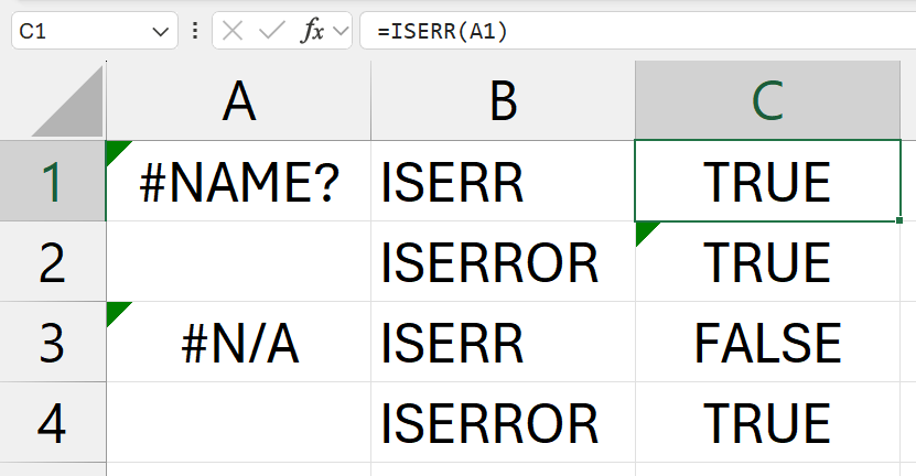
ISERR
Syntax: =ISERR(value)
Summary: Checks whether a value is an error other than #N/A, and returns TRUE or FALSE
Parameters:
value- might raise an error
Examples: Available at ISERROR
ISERROR
Syntax: =ISERROR(value)
Summary: Checks whether a value is an error, and returns TRUE or FALSE
Parameters:
value- might raise an error
Example:
Data Checking
Learn more:
Examples:
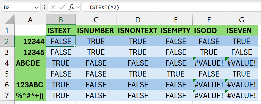
ISTEXT
Syntax: =ISTEXT(value)
Summary: TRUE if it only has text, else FALSE
Parameters:
value- a cell reference or a hard coded value
- this is what will be checked
ISNUMBER
Syntax: =ISNUMBER(value)
Summary: TRUE if it only has numbers, else FALSE
Parameters:
value- a cell reference or a hard coded value
- this is what will be checked
ISNONTEXT
Syntax: =ISNONTEXT(value)
Summary: Check if a value is not text. Blank cells are not text. Returns TRUE or FALSE accordingly.
Parameters:
value- a cell reference or a hard coded value
- this is what will be checked
ISBLANK
Syntax: =ISBLANK(value)
Summary: TRUE if its blank, else FALSE
Parameters:
value- a cell reference or a hard coded value
- this is what will be checked
ISODD
Syntax: =ISODD(value)
Summary: TRUE if it the number is odd, else FALSE
Parameters:
value- a cell reference or a hard coded value
- this is what will be checked
- must be a number
ISEVEN
Syntax: =ISEVEN(value)
Summary: TRUE if it the number is even, else FALSE
Parameters:
value- a cell reference or a hard coded value
- this is what will be checked
- must be a number
Text Manipulation
Learn more:
CONCAT
Syntax: =CONCAT(text, ...)
Summary: Concatenate/Join values together but with no seperation in middle. (like print(*args, sep="") in Python)
Parameters:
text- any cell references
- ranges
- but will get no space at middle (sep)
- individual cells
- ranges
- hardcoded characters
- anything...
- any cell references
Examples:
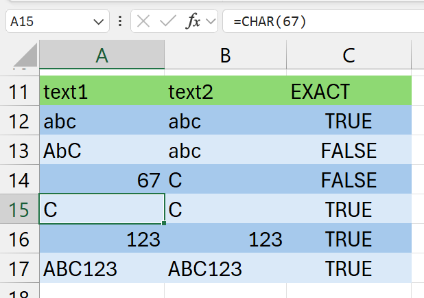
=CONCAT(a15, " ", b15)
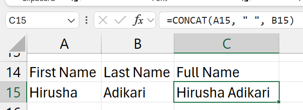
- contents of
a15+" "contents ofb15
LEFT
Syntax: =LEFT(text, [num_chars])
Summary: Get the left most characters of a selected value.
Parameters:
text- a single cell reference or a hard coded value
- to extract the characters from
num_chars- the number of characters to extract
- start counting from 1 (not from 0, like in programming languages)
Examples:
- assume
a1has ABCD1290
=LEFT(a1, 4)
- would result in:
ABCD
RIGHT
Syntax: =RIGHT(text, [num_chars])
Summary: Get the right most characters of a selected value.
Parameters:
text- a single cell reference or a hard coded value
- to extract the characters from
num_chars- the number of characters to extract
- start counting from 1 (not from 0, like in programming languages)
Examples:
- assume
a1has ABCD1290
=RIGHT(a1, 4)
- would result in:
1290
LEN
Syntax: =LEN(text)
Summary: Count the number of characters. Like the len() function in Python.
Parameters:
text- a single cell reference or a hard coded value
- to count the number of characters of
- if this cell
- has a text
- no. of characters in text is counted
- has a number
- no. of characters in number is counted
- has a formula
- no. of characters in the result is counted
- has a text
Examples:
=RIGHT(a2, LEN(a2)-3)
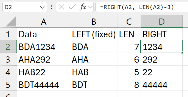
- in this example
- the length of numeric part changes
- so, to get the
RIGHTpart of it - we use the
LENfunction
- stages
LEN(a2)-3->7-3-> 4=RIGHT(a2, 4)-> get the right most 4 characters
FIND
Syntax: =FIND(find_text, within_text, [start_num])
Summary: Find for something and return it's index.
Parameters:
find_text- what character / set of characters to search for
within_text- where to search
start_num- optional
- defaults to 0 (from very first character)
- which charater to start counting from
- if 0, and starts with "
- if 1, and starts with "
- optional
Examples:
=FIND(" ", a2)
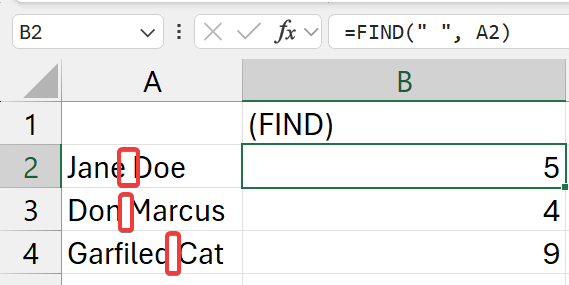
- find for a "
a2
=LEFT(A2, B2)
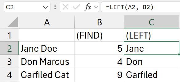
- get the first name
b2is the cell with the index of the "
=RIGHT(A2, LEN(A2)-B2)
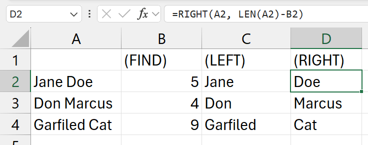
- get the last name
- similiar to the example of the
LEN function
MID
Learn more:
Syntax: =MID(text, start_num, num_chars)
Summary: Returns characters from the middle, given a starting position and length
Parameters:
text- source text to use
- can be a single cell reference or a hardcoded value
- works with both numbers and strings
start_num- index of the character to go to
- bring the pointer here (from left)
- value at his index is inclusive to our selection/stripping
num_chars- and move the pointer this many times to the right (from left)
Basically, num_chars characters starting from the start_num index of text (from left to right, as usual)
Examples:
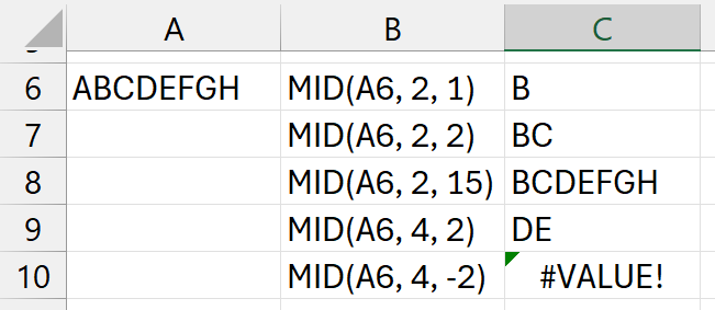
num_charsbeing negative- doesn't mean it will
- go from right to left
- it will error out (eg:
C10)
UPPER
Syntax: =UPPER(value)
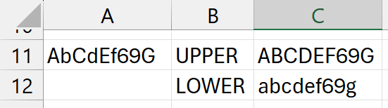
Summary: Converts a text string to all uppercase letters. Numbers will remain as it is.
Parameters:
value- a cell reference or a hard coded value
- this is what will be converted
Examples: Mentioned in the example with LOWER function
LOWER
Syntax: =LOWER(value)
Summary: Converts a text string to all lowercase letters. Numbers will remain as it is.
Parameters:
value- a cell reference or a hard coded value
- this is what will be converted
Examples:
=UPPER(A11) and =LOWER(A11)
EXACT
Syntax: =EXACT(text1, text2)
Summary: Checks whether two values are exactly the same and returns TRUE or FALSE accordingly. This is case sensitive.
Parameters:
text1- first value to compare
text2- second value to compare
Examples:
Lookup (Basic)
VLOOKUP
Learn more:
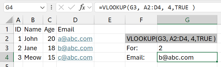
Syntax: =VLOOKUP(lookup_value, table_array, col_index_num, [range_lookup])
Summary: Look for a value (leftmost column of the table) and returns a value in the same row of a column you specify. By default, the table must be in ascending order. The table should be a normal vertical table.
Parameters:
lookup_value- what to search for
- in the table, the column with this value should be in the leftmost column of the table
- (if its to the right or middle, you should use
INDEX(MATCH)for it)
table_array- the table
- eg:
Client.csv!$A$2:$B$10- means, select table from
A2:B10 - with absolute cell referencing
- from Client.csv
- (in the current working directory)
- means, select table from
col_index_num- how many columns to go to right
- from the 1st column of the table
[range_lookup]- possible values
TRUE- Approximate Match
- no idea what this is
FALSE- Exact Match
- just use this
- possible values
Example:
=VLOOKUP(G3, A1:D4, 4, TRUE)
HLOOKUP
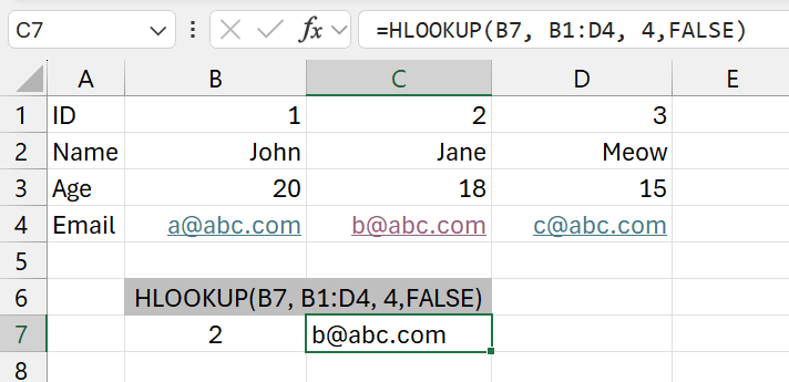
Syntax: =HLOOKUP(lookup_value, table_array, row_index_num, [range_lookup])
Summary: Look for a value in the top(most) row of a table (or an array of values) and returns the value in a same column of a row you specify (from the index). The table should be a weird horizontal table.
Parameters:
lookup_value- what to search for
- in the table, the row with this value should be in the top row of the table
- (if its to the bottom or middle, you should use
INDEX(MATCH)for it - but i have no idea about using it with a horizontal table... uhhhh)
table_array- the table
row_index_num- how many rows to go to bottom
- from the 1st row of the table
[range_lookup]- possible values
TRUE- Approximate Match
- no idea what this is
FALSE- Exact Match
- just use this
- possible values
Example:
=HLOOKUP(B7, B1:D4, 4, FALSE)
XLOOKUP
Syntax: =XLOOKUP(lookup_value, lookup_array, return_array, [if_not_found], [match_mode], [search_model])
Summary: Searches a range or an array for a match and returns the corresponding item from a second range or array. By default, an exact method is used. We can also pass values to return if not found. Can be used for both normal vertical tables and weird horizontal tables.
Parameters:
lookup_value- what to search for
lookup_array- where to search for the
lookup_value(a row) - search for value and get its index (
X)
- where to search for the
return_array- value we are looking from will be returned from this row
- return the item at the
Xindex of this row
if_not_found- return this value if no result is found
match_mode- possible values
-1: exact match or next smaller item0: exact match1: exact match or next larger item2: wildcard character match
- possible values
search_model- possible values
-2: binary search (sorted descending order)-1: search last to first1: search first to last2: binary search (sorted ascending order)
- possible values
Examples:
=XLOOKUP(F3, D2:D4, B2:B4, "Not Found")
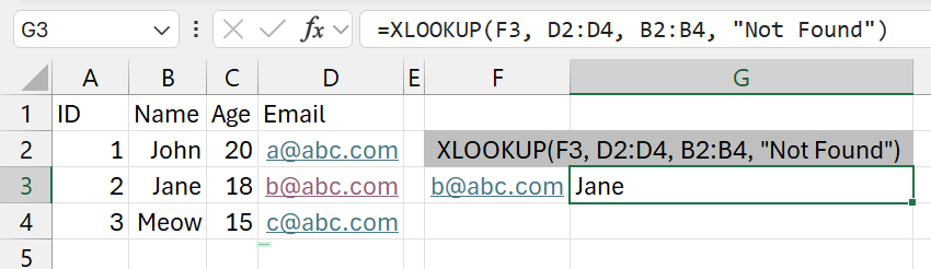
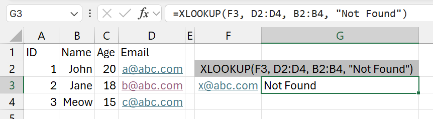
- We are searching from a column to the right compared to the column we are getting the result from.
Lookup (Advanced)
INDEX
Syntax: =INDEX(array, row_num, [col_num], ...)
Summary: Get the value in a selected cell range using an index for columns and rows. Value from Index
Parameters:
array- cell reference range
- either one dimentional (only a row or a column)
- or two dimentional (a table)
row_num- number of row
- start countng from 1
col_num- optional
- only if
arrayis two dimentional (a table)
- only if
- number of column
- start countng from 1
- optional
Examples:
=INDEX(b2:b10, 6)
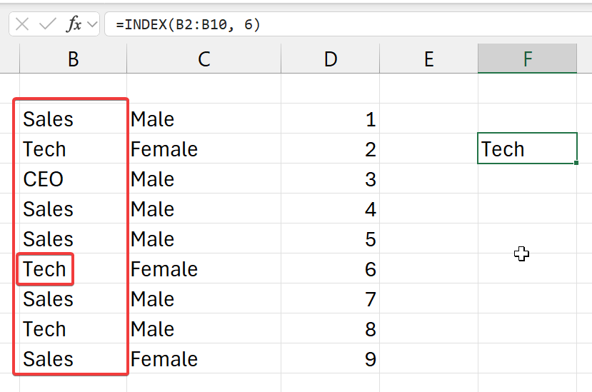
- from the top left corner (of selected row)
- go 6 cells down (rows)
- and get its value
=INDEX(b2:d4, 2)
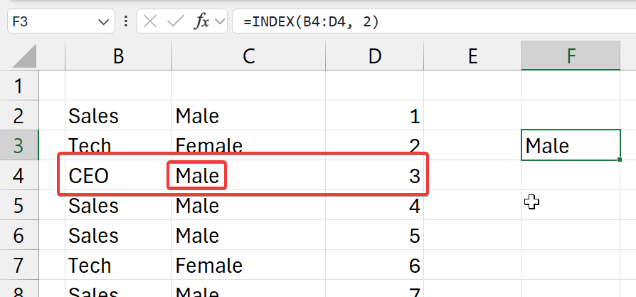
- from the top left corner (of selected column)
- go 2 cells right (columns)
- and get its value
=INDEX(b2:d10, 3, 2)
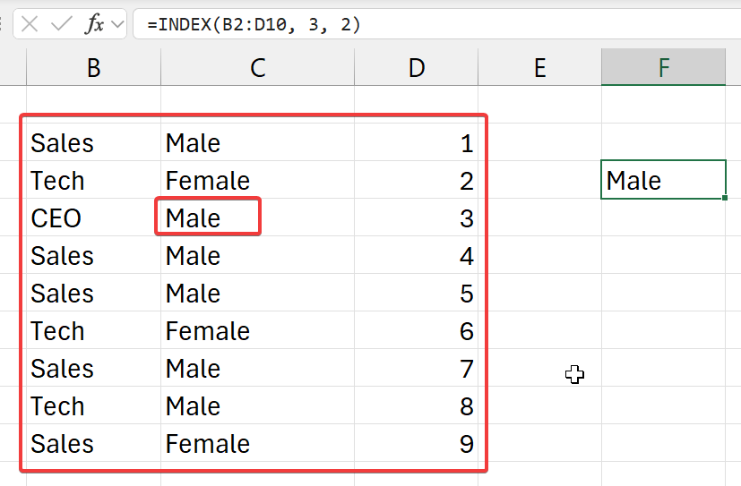
- (this proves that it doesn't count from A1)
- from the top left corner (of selected array of cells)
- go 3 cells down (rows)
- go 2 cells right (columns)
- and get the value at that index
- from this selected table
OFFSET (Basic)
Syntax: =OFFSET(refernce, rows, cols)
Summary: Get the value at an offset of rows and columns from a selected cell. Value from Index
Parameters:
array- cell to start moving from
rows- number of rows to go down
cols- number of columns to go right
Examples:
=OFFSET(b3, 3, 1)
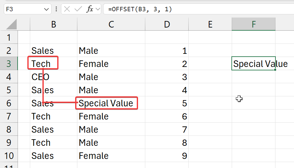
- start from cell
b3- go 3 cells down (rows)
- go 1 cell right (columns)
- and get that value
OFFSET (Advanced)
Syntax: =OFFSET(refernce, rows, cols, [height], [width])
Summary: Get the value at an offset of rows and columns from a selected cell. Value from Index
Parameters:
array- cell to start moving from
rows- number of rows to go down
cols- number of columns to go right
Examples:
=OFFSET(b3, 3, 1, 3, 2)
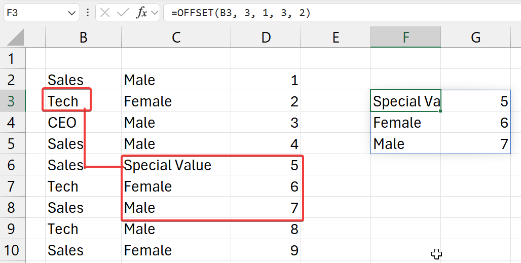
- start from cell
b3- go 3 cells down (rows)
- go 1 cell right (columns)
- and get values
- of 3 rows
- and 2 columns
Compound usage: these functions are used with another function most of the time.
=SUM(OFFSET(b3, 3, 1, 3, 2))
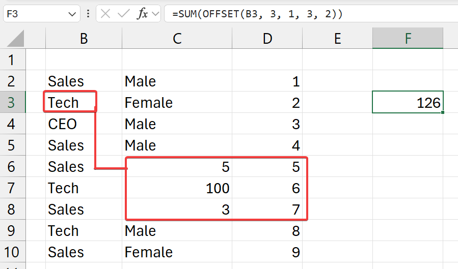
- start from cell
b3- go 3 cells down (rows)
- go 1 cell right (columns)
- and get values
- of 3 rows
- and 2 columns
- and
SUMall of it
MATCH
Syntax: =MATCH(lookup_value, lookup_array, match_type)
Summary: Get the index of a value in the specified cell reference range. Index from Value
Parameters:
lookup_value- what to search for
- index of this will be returned
lookup_array- where to search for
match_type- values
1: Less than0: Exact match-1: Greater than
- values
Examples:
=MATCH("CEO", b2:b10, 0)
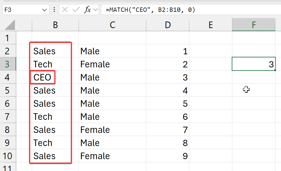
- select an exact match (
0) - from the selected cell range (column) (
b2:b10) - and get the index of where
CEOis to be found
=MATCH("Tech", b2:b10, 0)
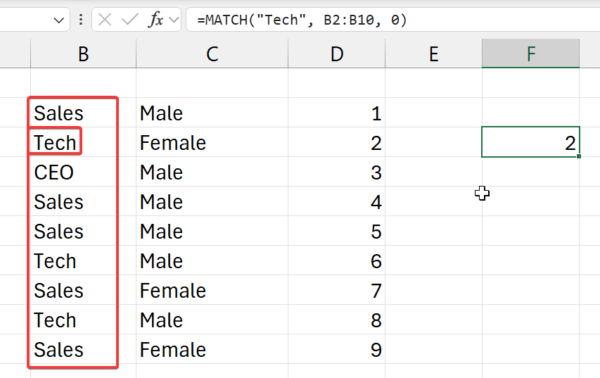
- select an exact match (
0) - from the selected cell range (column) (
b2:b10) - and get the index of where
Techis to be found - NOTE:
- can be found 3 times
- only the index of first time is given
INDEX(MATCH) Combined Usage
Example:
=INDEX(A1:D7, MATCH($G$2, B1:B7, 0), 3)
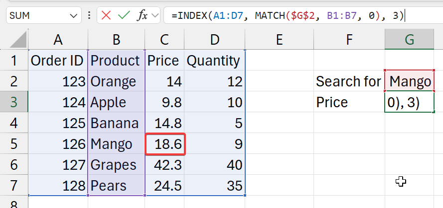
- where
$G$2is the search field (set with absolute cell referencing)A1:D7is the full table (with data), including titles3is the column with the pricing information
- functions breakdown
MATCH($G$2, B1:B7, 0)- get (input) value from G2 cell
- look for and exact match for this (input) value
- in
B1:B7cell range- as the selected table also includes titles
- make sure select he titles here as well
- and get it's index
=INDEX(A1:D7, XXX, 3)- in the table
A1:D7- go
XXXnumber of cells down (from stage 1) (rows) - then, 3 cells to right (columns)
- go
- return its value
- in the table
BUT, in the above example, we hardcode the column index ourselves. It's hard to find it and we will have to change stuff if the column order is changed in the table. Also, we can lookup for other stuff (like Quantity) easily without having to write new formulas. So, we will get the column index dynamically.
=INDEX(A1:D7, MATCH($G$2, B1:B7, 0), MATCH($G$1, A1:D1, 0))
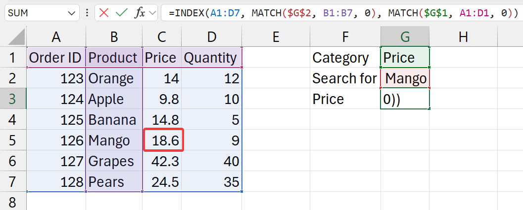
- where
$G$1is the catgeory field (set with absolute cell referencing). This mentions to catgeory to return from result.$G$2is the search field (set with absolute cell referencing). This mentions what to search for.A1:D7is the full table (with data), including titles3is the column with the pricing information
- functions breakdown
MATCH($G$2, B1:B7, 0)- get (input) value from G2 cell
- look for and exact match for this (input) value
- in
B1:B7cell range- as the selected table also includes titles
- make sure select he titles here as well
- and get it's index
MATCH($G$1, A1:D1, 0)- get (input) value from G1 cell
- look for and exact match for this (input) value
- in
A1:D1cell range (titles row)
=INDEX(A1:D7, XXX, YYY)- in the table
A1:D7- go
XXXnumber of cells down (from stage 1) (rows) - then,
YYYcells to right (from stage 2) (columns)
- go
- return its value
- in the table
CS Data Types Stuff
Examples:
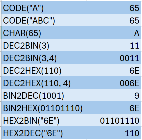
CODE
Syntax: =CODE(value)
Summary: Returns the numeric code for the first character in a text string. Numeric code will be from the character set used by the computer.
Parameters:
value- a single cell reference or a hard coded value
- if it has many characters
- only the first character is considered/used
CHAR
Syntax: =CHAR(value)
Summary: Returns the character specified by the code number from the character set of your computer.
Parameters:
value- a single cell reference or a hard coded value
DEC2BIN
Syntax: =DEC2BIN(number, [places])
Summary: Convert a decimal number to binary form.
Parameters:
number- a single cell reference or a hard coded value
- a number
- this number is what will be converted
places- like the word length
- add zeros to the front
- to get the binary number to the required length
DEC2HEX
Syntax: =DEC2HEX(number, [places])
Summary: Convert a decimal number to hexadecimal form.
Parameters:
number- a single cell reference or a hard coded value
- a number
- this number is what will be converted
places- like the word length
- add zeros to the front
- to get the hex number to the required length
BIN2DEC
Syntax: =BIN2DEC(number)
Summary: Convert a binary number to decimal form.
Parameters:
number- a single cell reference or a hard coded value
- a number
- this number is what will be converted
BIN2HEX
Syntax: =BIN2HEX(number, [places])
Summary: Convert a binary number to hexadecimal form.
Parameters:
number- a single cell reference or a hard coded value
- a number
- this number is what will be converted
places- like the word length
- add zeros to the front
- to get the hex number to the required length
HEX2BIN
Syntax: =BIN2HEX(number, [places])
Summary: Convert a hexadecimal number to binary form.
Parameters:
number- a single cell reference or a hard coded value
- a number
- this number is what will be converted
places- like the word length
- add zeros to the front
- to get the hex number to the required length
HEX2DEC
Syntax: =HEX2DEC(number)
Summary: Convert a hexadecimal number to decimal form.
Parameters:
number- a single cell reference or a hard coded value
- a number
- this number is what will be converted
Datetime
Cells with date(time) can be added, subtracted to calculate timedeltas.
Maybe keep everything in the same format as a good practice.
Examples:
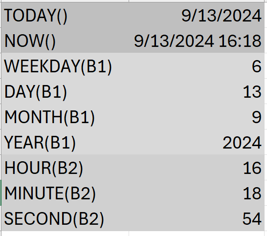
- (
WEEKDAY-> 6 -> means its "Friday")
TODAY
Syntax: TODAY()
Summary: Return the current date formatted as a date
Parameters: None
NOW
Syntax: NOW()
Summary: Return the current date and time formatted as a date and time
Parameters: None
WEEKDAY
Syntax: WEEKDAY(serial_number, [return_type])
Summary: Return the current date and time formatted as a date and time
Parameters:
serial_number- a cell reference with a date
- either custom date(time) and formatted
- or from
NOW() - or from
TODAY()
- a cell reference with a date
return_type- optional
- defaults to 1
- just dont touch it
- it will change the order of how dates are indexed (scope: this usage of the function only)
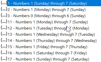
- we will be sticking to the default thing
Examples:
- Days and numbers returned in this order:
Sunday->1Monday->2...Friday->6Saturday->7
DAY
Syntax: DAY(serial_number)
Summary: Return the day of a month. A value from 0 to 31
Parameters:
serial_number- a cell reference with a date
- either custom date(time) and formatted
- or from
NOW() - or from
TODAY()
- a cell reference with a date
MONTH
Syntax: MONTH(serial_number)
Summary: Return the month. A number from 1 (January) to 12 (December)
Parameters:
serial_number- a cell reference with a date
- either custom date(time) and formatted
- or from
NOW() - or from
TODAY()
- a cell reference with a date
YEAR
Syntax: YEAR(serial_number)
Summary: Returns the year of a date. An integer in the range 1900 - 9999
Parameters:
serial_number- a cell reference with a date
- either custom date(time) and formatted
- or from
NOW() - or from
TODAY()
- a cell reference with a date
HOUR
Syntax: HOUR(serial_number)
Summary: Returns the hour as a number. From 0 (12:00 AM) to 23 (11:00 PM)
Parameters:
serial_number- a cell reference with a date and time
- either custom datetime and formatted
- or from
TODAY()
- a cell reference with a date and time
MINUTE
Syntax: MINUTE(serial_number)
Summary: Returns the minute. A number from 0 to 59.
Parameters:
serial_number- a cell reference with a date and time
- either custom datetime and formatted
- or from
TODAY()
- a cell reference with a date and time
SECOND
Syntax: SECOND(serial_number)
Summary: Returns the second. A number from 0 to 59.
Parameters:
serial_number- a cell reference with a date and time
- either custom datetime and formatted
- or from
TODAY()
- a cell reference with a date and time
DATEDIF
Not in Microsoft Office: Excel 2021 LTS.
Statistics
MEAN ??
Learn more at the Average section
MEDIAN
Syntax: =MEDIAN(range, [range2], ...)
Summary: Median of everything in the selected range(s).
Paramaters:
range- range to calculate median of.
- eg:
c1:c9
[range2]- other ranges to calculate median of
Examples:
a1:a9is job descriptionsb1:b9is genderc1:c9is salary
=MEDIAN(c1:c9)
- median of all numerical values in range
c1:c9
MODE
Syntax: =MODE(range, [range2], ...)
Summary: Mode of everything in the selected range(s).
Paramaters:
range- range to calculate mode of.
- eg:
c1:c9
[range2]- other ranges to calculate mode of
Examples:
a1:a9is job descriptionsb1:b9is genderc1:c9is salary
=MODE(c1:c9)
- Mode of all numerical values in range
c1:c9
SUBTOTAL
Lean more:
Syntax: =SUBTOTAL(function_num, range1, [range2], ...)
Summary: Basically select and perform a a function from a list of functions to a selected range. You can calculate the sum, average, or anything else from the 15+ other choices.
Paramaters:
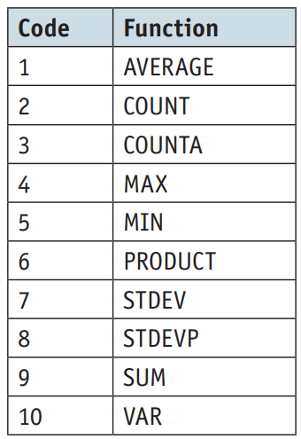
function_num- what function to actually perform
- in a number
- just select from the drop down menu
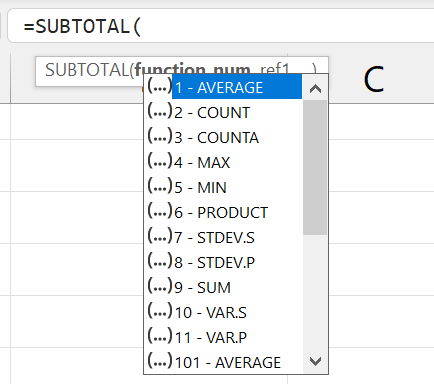
- REMEBER THESE FOR PAPER 1
range1- range to perform the calculation.
- eg:
c1:c9
[range2]- other ranges to perform the calculation.
Examples:
a1:a9is job descriptionsb1:b9is genderc1:c9is salary
=SUBTOTAL(9, c1:c9)
- Sum everything in
c1:c9 - similiar to running
=SUM(c1:c9)
=SUBTOTAL(101, c1:c9)
- Average everything in
c1:c9 - similiar to running
=AVERAGE(c1:c9)